As it turns out, mapping in R is (almost) totally easy!
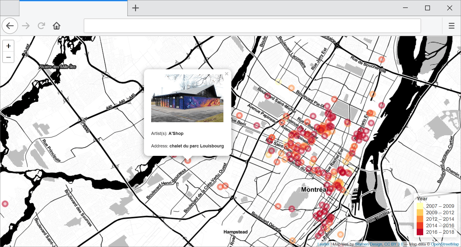
Some months ago, I found a dataset of all of the locations of Montreal’s publicly commissioned murals on the city’s open data portal. As someone who has very much enjoyed many of these murals, I’ve been looking forward to creating an interactive web map with this data for quite a while. My recent foray into the world of spatial analysis in R (thanks to my GIS module this semester) showed me a simple way to create a basic, but quite nice looking, web map using the Leaflet library for R.
So here’s how it was done:
I first loaded the Leaflet, readr, and classInt libraries. After downloading the CSV dataset from Montreal’s portal, I read this file into R.
murals <- read_csv("Montreal/murals.csv")
This dataset contains the lat/long position for a total of 203 murals with a number of attributes, including year, artist, and a link to a photo of the mural.
In addition to plotting the location of each of the murals on a map, I wanted to colour the markers differently according to the year that the mural was painted. To do this, I first created a colour palette with values/colours separated according to the Jenks natural breaks approach.
# make breaks in the data
breaks<-classIntervals(murals$annee,
                       n=5,
                       style="jenks")

# just keep the break values
breaks <- as.numeric(breaks$brks)

# create new  colour palette
pal <- colorBin(palette = "YlOrRd",
				# these are the years values in the dataset
                domain = murals$annee,
                #create bins using the breaks object from earlier
                bins = breaks)
Now all that was left to do was plot the data on a map! Two elements of this required a bit of problem-solving. First, I wanted to create some nice pop-ups for each mural point to display the photo of the mural (from the URL provided in the dataset), its artist(s), and the address of the mural. All of this information was included in the CSV that I downloaded. Thanks to StackOverflow, I discovered how to add in some HTML code to customize the popups for my markers.
The second challenging element had to do with formatting the legend. In reading each of the year values as numbers, R displayed the values in the legend labels with some annoying commas (eg. 2,009 vs 2009). It took quite a bit of fiddling around to figure out how to change the default formatting to remove this comma.
# make a murals map
murals_map <- leaflet(murals) %>%
  # add in the markers for each mural
  addCircleMarkers(radius = 7, lng = ~longitude, lat = ~latitude, popup = paste0("<img width = '200px'; src = ", murals$image, "><p>Artist(s): <b>", murals$artiste, "</b></p><p>Address: <b>", murals$adresse, "</b></p>"), color = ~pal(annee)) %>%
  # add the basemap
  addProviderTiles(providers$Stamen.Toner) %>%
  addLegend("bottomright",
            pal= pal,
            values = ~annee,
            title = "Year",
            opacity = 1,
            # change the default number formatting in the legend to get rid of the comma
            labFormat = labelFormat(big.mark = "")
  )
Follow this link to check out the full interactive version of this map. Some of this code is adapted from Chapter 2 of our CASA0005 practical book.
Check out the full code for this exercise here