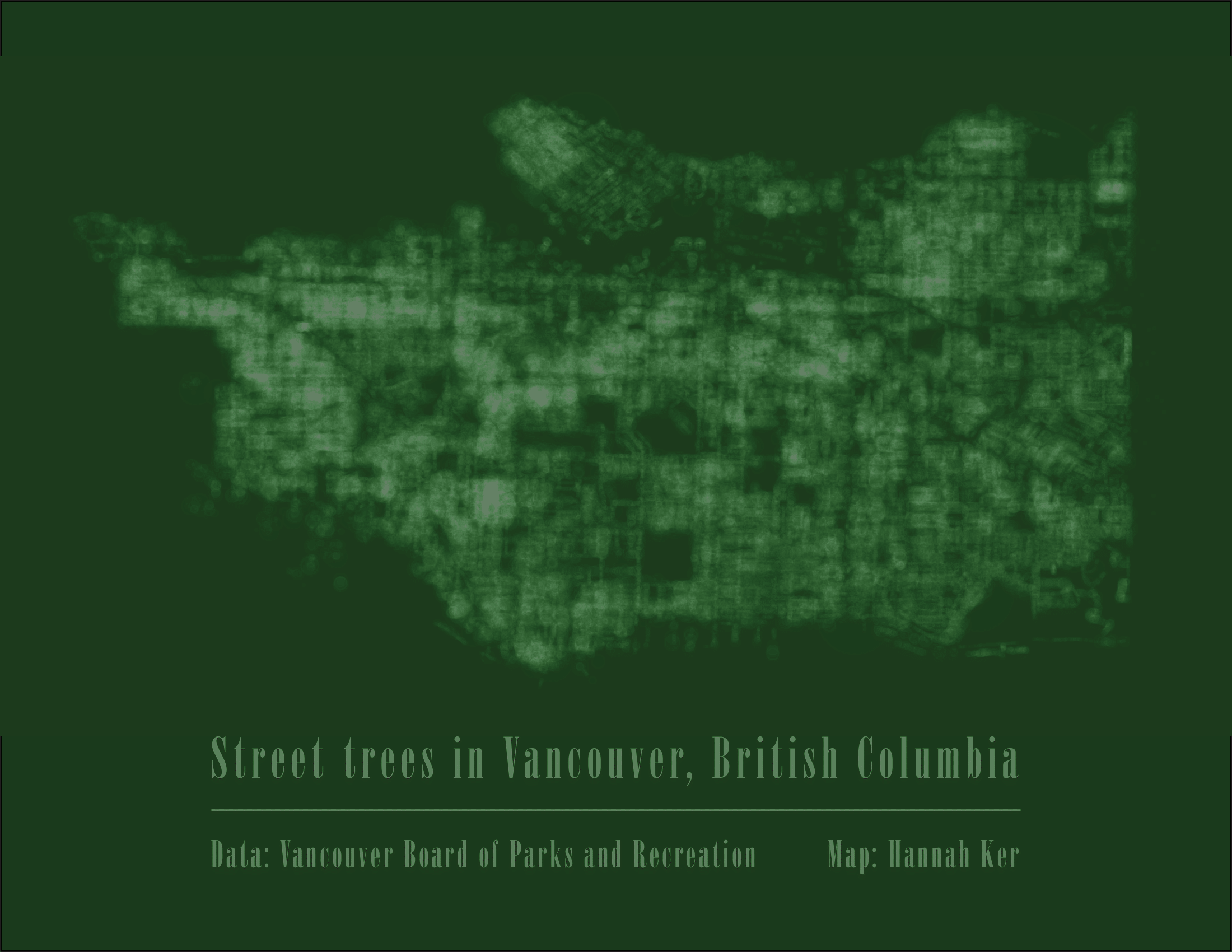
I have been a long-time admirer of the ‘Minimal Maps’ series from Michael Pecirno, and wanted to try to recreate something similar. I really liked his focus on the natural environment and spent a while exploring potential datasets, at a variety of scales. I eventually settled on this dataset of street trees in Vancouver. This dataset has one point for every public tree on Vancouver’s boulevards (there are over 140,000!).
Data Cleaning 
I downloaded this dataset as a CSV (it was taking too long to open in R as a GeoJSON) and read it into R.
# loading in necessary libraries
library(ggplot2)
library(rlist)
library(sf)

# open the dataset
trees <- read.csv('street-trees.csv', sep = ';')
Because I am still finding R’s factor data type challenging to work with, I converted everything into integers or strings. I also removed the entries without any coordinates.
# convert factors to strings
i <- sapply(trees, is.factor) # find columns that are factors
trees[i] <- lapply(trees[i], as.character) # convert column to character

# remove rows without coordinates
new <- subset(trees, nchar(Geom) > 1)
The most challenging part of this process was getting the coordinate data into a workable format. Initially, this data for each tree was stored in a cell in a format like this:
{"type": "Point", "coordinates": [-123.135032, 49.230858]}
I wrote a function to parse these strings, one at a time, and return a list that contained just the coordinates.
# function to parse strings to get coordinates
getcoords <- function(string){

  split <- strsplit(string,']')[[1]]
  a <- split[[1]]
  b <- strsplit(a, '-')[[1]][[2]]
  c <- strsplit(b, ',')
  d <- c[[1]]

  x <- paste0('-', d[[1]])
  y <- strsplit(d[[2]], ' ')[[1]][[2]]

  coords <- list(x,y)
  return(coords)

}
I applied this function to each point in the dataset and created new columns for each coordinate.
# apply the function for each row
for (i in 1:length(new$Geom)){

  # parse to get the coordinates
  z <- getcoords(new$Geom[[i]])
  x <- z[[1]]
  y <- z[[2]]

  # add new columns to df
  new$lats[i] <- x
  new$longs[i] <- y

}

# convert the columns from characters to nums
new$lats <- as.numeric(new$lats)
new$longs<- as.numeric(new$longs)
Visualizing the data 
Once all the data was cleaned, it was a very simple matter to visualize using ggplot2. Given that the dataset was decently large, I took a smaller subset of all points for faster visualization while I tested different visualization parameters.
# get smaller version for faster testing
small <- new[1:2500,]

# make the map
map <- ggplot(data=small) +
  geom_point(data=small,
             aes(x=small$lats,
                 y=small$longs),
             size=small$DIAMETER*0.1,
             alpha=0.005,
             color='#ffffff')+
  theme_map()
After outputting this map, I used inDesign to add some simple text for a title.