Overview
Using data collected from London’s ANPR camera system, I built and trained a machine learning model to predict travel times across 22 road links in central London.
The data
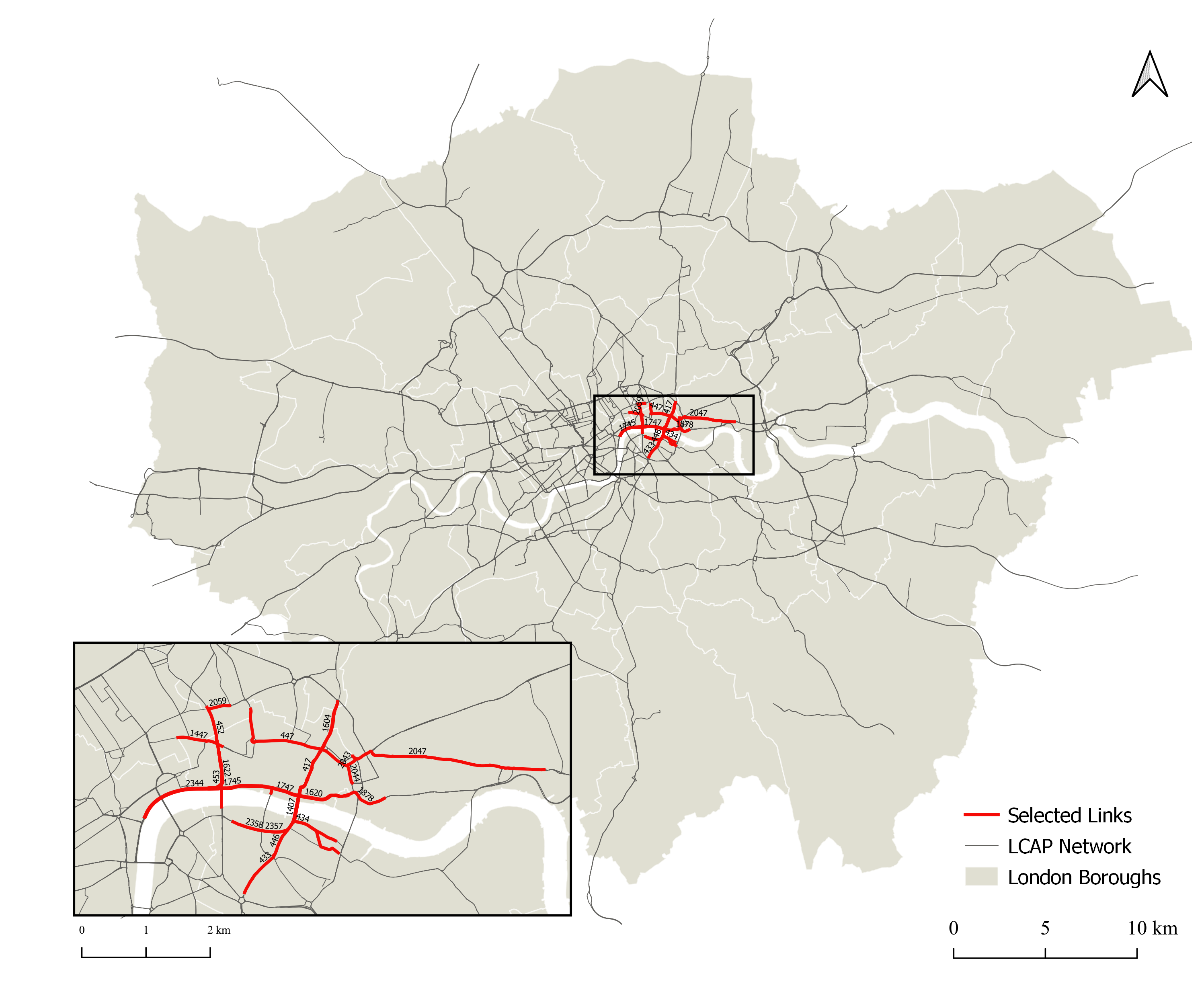
This data was collected as part of the London Congestion Analysis Project and provides travel times (in sec/meter), aggregated at 5 min intervals for road links throughout London. This data was collected between January 1st, 2011 and January 30th, 2011 and includes observations between 6am-9pm for each day. I focused my analysis by selecting a subset of 22 road links, as shown in the map below.
Modelling data with spatial and temporal dependencies
Traffic data is complex. As traffic is measured across both spatial and temporal dimensions, we need to consider the effects of spatial and temporal autocorrelation.1 That is, two traffic speed measurements are more likely to be similar to each other if they are closer in space and time. Many traditional statistical and machine learning methods are not designed to handle these effects, and so accurate predictions can be challenging.
To address this challenge, we need to first explore our data to understand its spatial and temporal patterns. Moran’s I is a useful measure of local spatial autocorrelation, indicating how each observation is correlated with its neighbours. We can also create ACF and PACF plots to understand how each observation is correlated with its past observations.
Methods
Given its past applications in time series modelling and traffic predictions2,3 I used support vector regression (SVR) to create my model.
Support vector regression (SVR) is an adapted version of the popular support vector machine (SVM) model, that is used to solve regression, rather than classification problems. Both SVR and SVM are kernel methods. Generally speaking, kernel methods function in two steps.4 Firstly, a function is applied to map the data into a high dimensional feature space. Then, a learning algorithm is applied to find linear patterns in this feature space.4 Well-established linear algorithms (eg. OLS regression) can thus be applied so solve nonlinear problems.
I used the caret package in R to develop the SVR model and use the MLmetrics package to calculate metrics to evaluate its performance. Given the results from our data exploration, we built a model that incorporated 3 time lags (ie. the past three observations) to predict the next time step. As I identified statistically significant spatial autocorrelation (as identified by a Moran’s I test), I tested models that included information from spatially adjacent links, but found that this increased training time and did not significantly improve model accuracy.
I then split the data into training and testing sets, encompassing 16 days of observations and 7 days of observations, respectively. Using the testing set, I used a grid search approach to tune the hyperparameters for the SVR model. These hyperparameters control factors such as the model’s sensitivity to error and the bandwidth for the kernel function that this model is based on (RBF kernel, in this case). For greater efficiency, I only tuned the hyperparameters based on the data from a single road link (rather than for all 22). Using the optimal combination of hyperparameters, I created an SVR model and applied it to the testing data for all road links to make travel time predictions.
Results
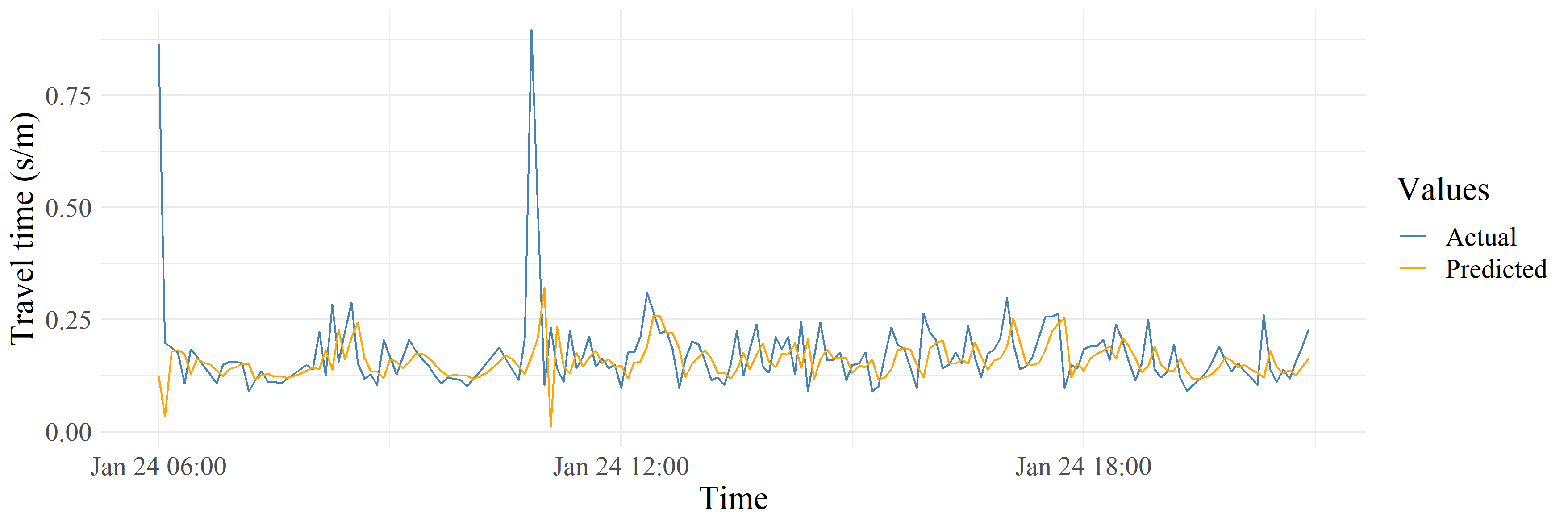
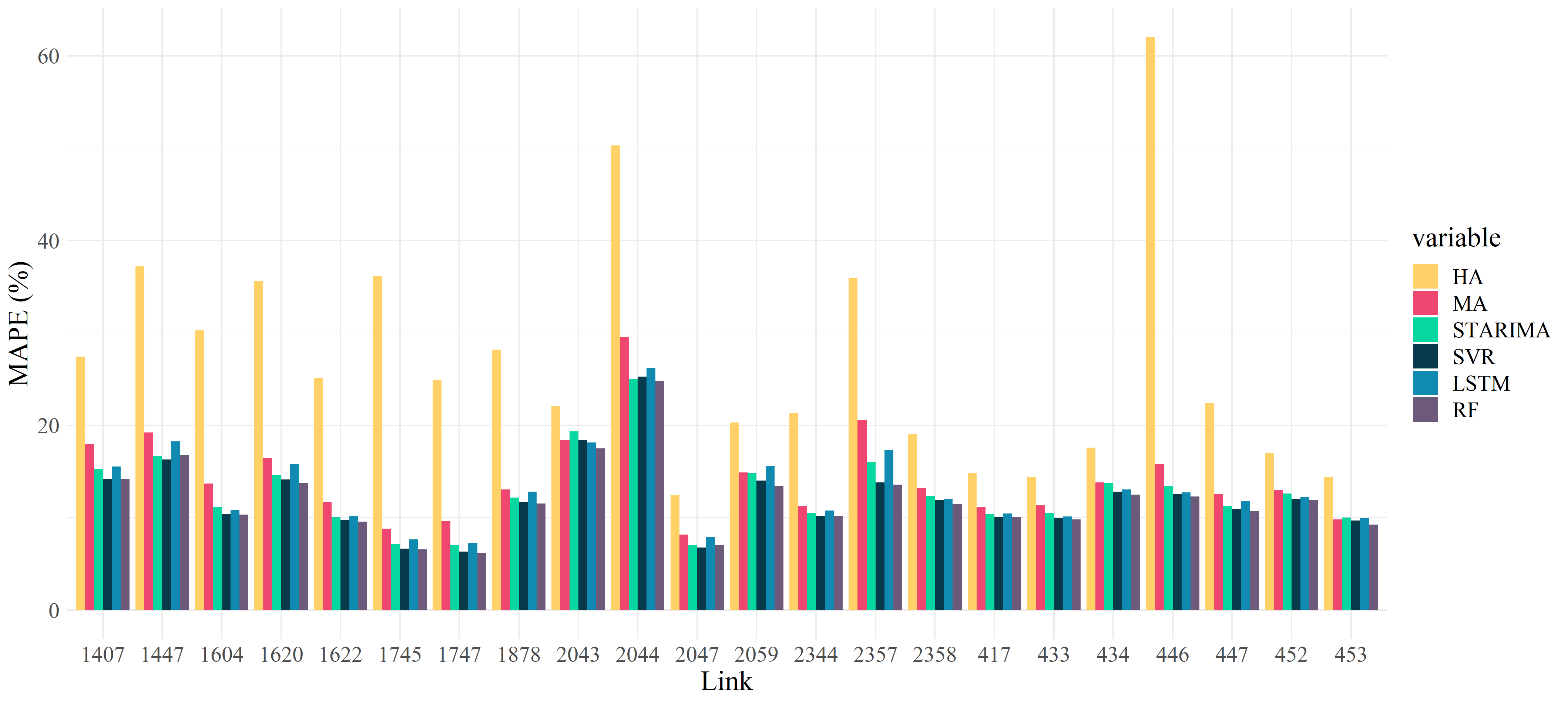
The figure at the top of this post gives an example of the actual travel times in the dataset, compared with the travel times predicted by my model. When looking at this model’s error (as measured by MAPE), according to the figure below, we can see that this SVR traffic prediction model performs competitively against other state-of-the-art approaches, such as STARIMA (a spatio-temporal extension of the traditional ARIMA time series model), and long short-term memory (a deep learning approach). These other models were created by other students in my course, with the same data.
Admittedly, this model may be of limited utility, as travel time predictions are only made 5 minutes in the future. Nonetheless, it is an interesting exercise in exploring different approaches for building predictive models that are somewhat robust to underlying spatial and temporal dependencies in the data.
- Cheng, T., Haworth, J., Wang, J., 2011a. Spatio-Temporal Autocorrelation of Road Network Data. J. Geogr. Syst. 14, 1–25. https://doi.org/10.1007/s10109-011-0149-5 [return]
- Müller, K.-R., Smola, A.J., Rätsch, G., Schökopf, B., Kohlmorgen, J., Vapnik, V., 1999. Using support vector machines for time series prediction, in: Advances in Kernel Methods: Support Vector Learning. MIT Press, Cambridge, MA, USA, pp. 243–253. [return]
- Wu, C.-H., Ho, J.-M., Lee, D.T., 2004. Travel-time prediction with support vector regression. IEEE Trans. Intell. Transp. Syst. 5, 276–281. https://doi.org/10.1109/TITS.2004.837813 [return]
- Shawe-Taylor, D. of C.S.R.H.J., Shawe-Taylor, J., Cristianini, N., 2004. Kernel Methods for Pattern Analysis. Cambridge University Press. [return]